At the Snowflake Summit this year, Snowflake introduced Snowpark — a library for processing data in your warehouse with the languages, code, and scientific tools you already use.
As hundreds of teams use Snowflake with Deepnote to explore and build data products, we used this opportunity to make the Snowflake and Deepnote experience even more delightful.
In this article, we'll walk you through what makes Snowpark such a valuable asset for data science workflows and show how you can use its superpowers in Deepnote — Snowpark’s Python-ready partner.
Let’s dive in!
The toolbox
We are using Deepnote notebooks as a control plane for our Snowflake warehouse. Deepnote is a collaborative data workspace for data science and analytics — it allows for real-time collaboration, integrates with Snowflake seamlessly with SQL blocks, and enables rapid exploration and prototyping with Python. This way we benefit from the agility of a notebook's interface and Snowflake’s security, scalability, and compute.
Snowpark & Deepnote 101
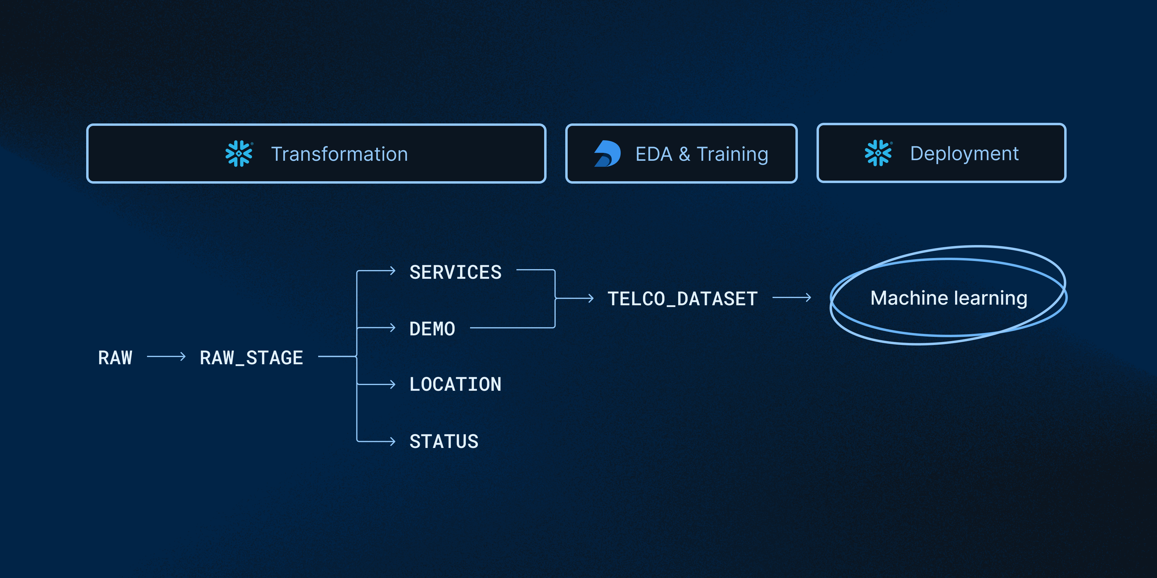
The goal of this tutorial is to build an end-to-end data science pipeline — from transformation to data exploration to model training and evaluation to model deployment. The sample data set, which we will build ML models with later, contains 100K rows of telecommunications data. The full pipeline looks something like this:

👉 If you want to play with the integration right away, you can find a template and a detailed version of this walkthrough in this notebook.
1. Setting up Snowflake in Deepnote
In this section, we'll use Snowpark to connect to and populate our Snowflake warehouse.
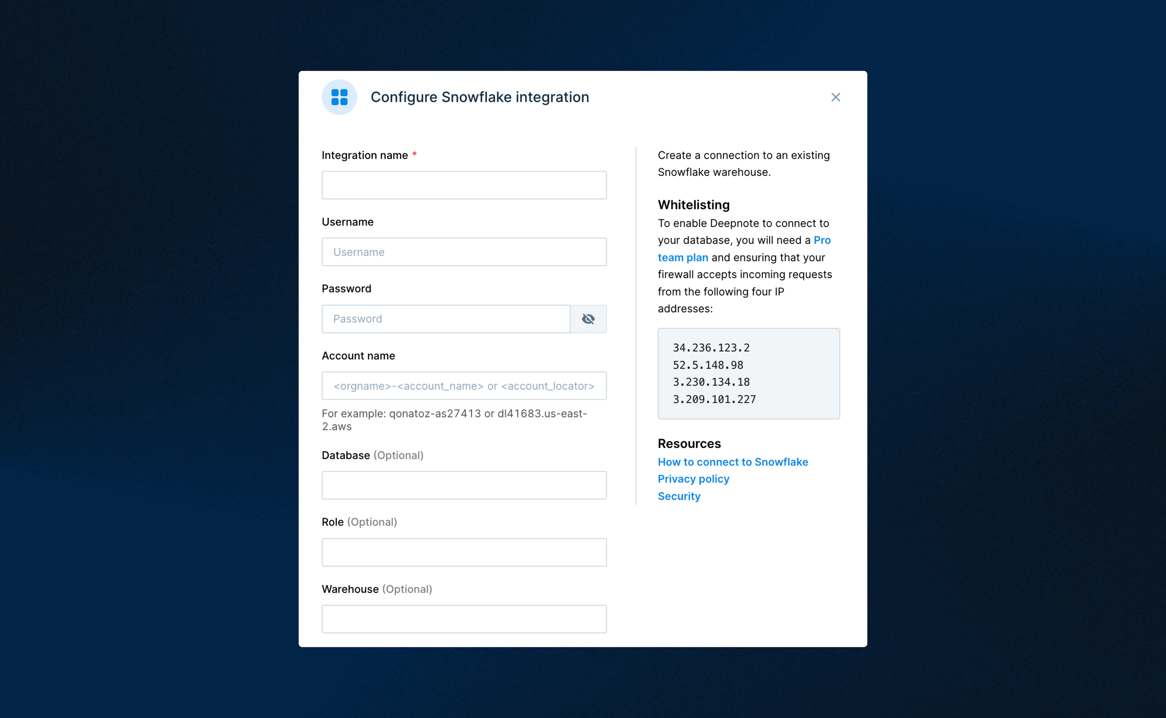
First, we establish a data connection with Snowflake from Deeponote. If you don’t have a Deepnote account, you can create one for free here. Your credentials are kept secret with Deepnote’s environment variables integration, and the connection can be shared and reused across your team’s workspace.

If you're starting this demo from scratch, you'll also need to set your Python environment to Python 3.8 (use the settings in the right side bar to access Deepnote's environments). The rest of the nitty-gritty setup and authentication details are best viewed in the full notebook walkthough here.
Once the setup is complete, we then create the session object, which allows us to interact with the Snowflake warehouse via its pandas-like API. Simply pass your connection details to the config method to connect to your Snowflake instance.
We're using a sample telecommunications data set, a parquet file containing approximately 100K rows that is bundled with the notebook. Using the session object from Snowpark, we upload that file as a table in our warehouse as shown below.
Let’s check out our new table by displaying it as an interactive Pandas DataFrame in Deepnote.
Now that we’ve set the stage, it’s time for data transformation as we work toward a dataset we can use for machine learning.
2. Data transformation
We begin by transforming our data with Snowpark’s main abstraction — the DataFrame, which contains methods for operating on the data. Importantly, all transformations are computed in the warehouse itself, not the notebook.
You could pass pure SQL to the session object, but by using the DataFrame in a notebook environment, we’re getting intelligent code autocomplete and error highlights in the notebook while benefiting from the speed.
Below is an overview of the data pipeline and respective transformations. We start with our raw table (loaded from the parquet file), build up several transformations, and finally land on a table that we can use to build a churn prediction model.

Below is an example of how the TELCO_DATASET was built using the DataFrame’s join method from Snowpark. Snowpark disambiguates the duplicate column in the joined table by prepending a random string to the original column name. Chaining a new select statement gives us back a column simply called CUSTOMERID.
Now we have a table the data scientists can use for machine learning. Specifically, we’re going to use scikit-learn to build a churn prediction model based on the TELCO_DATASET table.
3. Exploratory data analysis
Once we’ve completed the transformations, our freshly minted TELCO_DATASET can be used for model training and prediction. We will first do the requisite exploratory data analysis to make sure our data set is suitable for model training. We examine the data for missing values, outliers, or anything else that might affect our subsequent modeling.
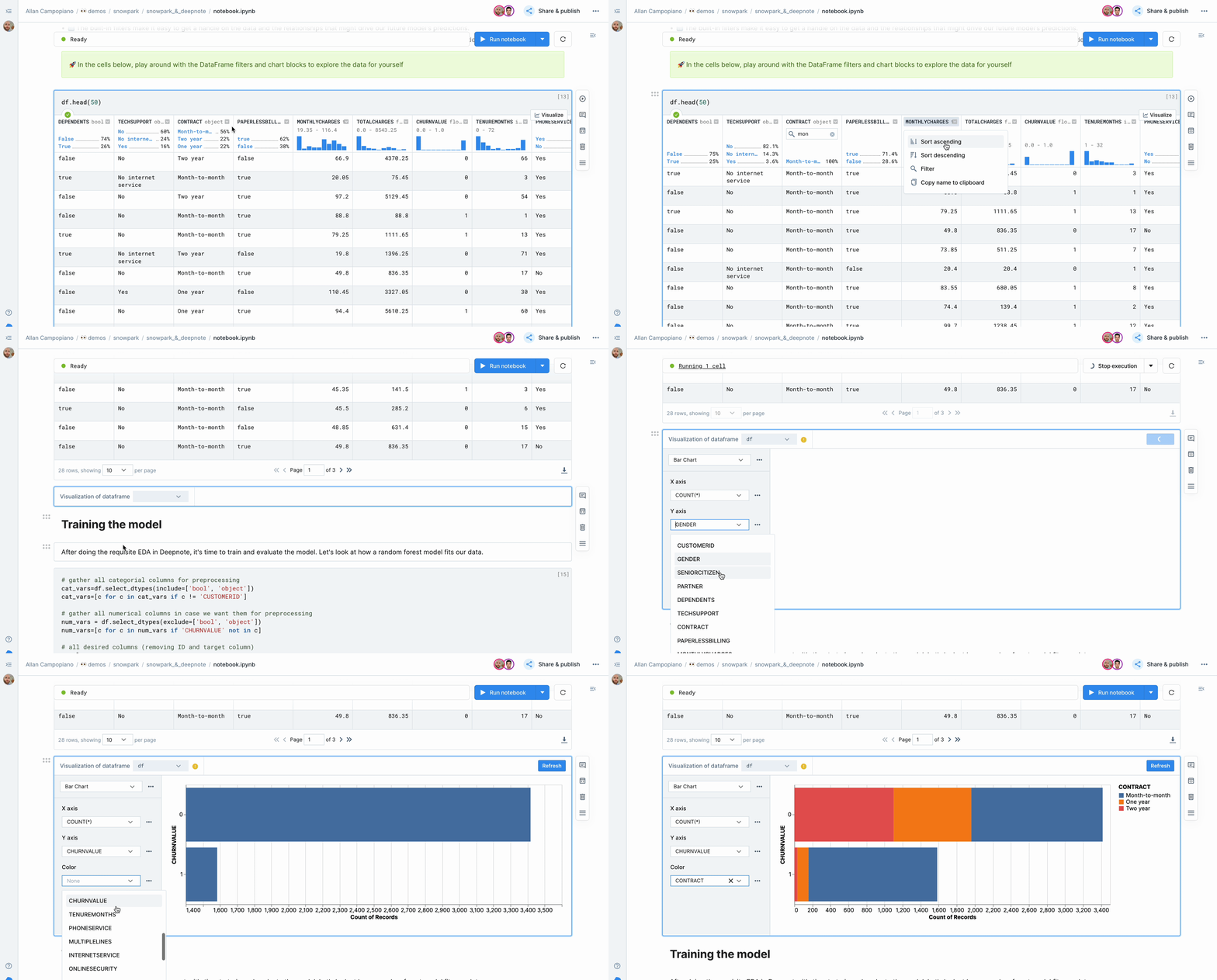
In Deepnote, a great deal of the exploratory work happens without writing any code thanks to some built-in EDA magic, such as rich DataFrames, built-in sorting and filters, and no-code charts. This way, we can examine the data set for data types, missing values, percentage of given categories, distributions, and more, shifting seamlessly from code to visualizations to querying and back.

4. Model training
After doing the requisite EDA in Deepnote, we can train and evaluate the model. We applied a random forest classifier and took a look at the confusion matrix to evaluate the accuracy of the classifications.
After evaluating our model's accuracy, we can now deploy this model directly on the Snowflake warehouse without changing our code or package environment. Moreover, any new data that ends up in our warehouse can be fed into the model to predict churn without having to take our data out of the warehouse.
5. Model deployment
In order to deploy models to Snowflake, we use Snowpark's powerful user-defined functions. UDFs are functions that are defined in pure Python but run on Snowflake compute. This is a perfect fit for our newly created model. They are decorated with @udf and require a few other details beyond a standard Python function. Read the Snowpark documentation to learn more.
Let’s use a Snowpark UDF to move our model onto the Snowflake server, where it can be used for predictions with incoming data.
The only thing left to do is use the model to make some predictions. We’ll take a sample from the TELCO_DATASET table to use for that.
The Snowpark select statement above accomplished the following tasks:
- It selected the
CUSTOMER_ID,CHURNVALUE, and the output of thepredict_churnfunction we wrote earlier (aliased toPREDICTED CHURN). - It saved the results set to a new table in our warehouse called
CHURN_DETECTION.
Now we can query the new CHURN_DETECTION table with Deepnote’s native SQL blocks to check it out.
We have sucessfully deployed and made predictions with our model on Snowflake without changing our code, package environment, or moving our data out of the warehouse.
Conclusion
With Deepnote and Snowpark, the entire database feels like an in-memory object, similar to the experience of using pandas, but at a much larger scale. All the transformation and scientific computation happen where the data lives, without having to change tools, libraries, or languages.
Whether you’re a data scientist, analytics engineer, data engineer, developer, or an analyst — if you’re using Snowpark, Deepnote will be a great addition to your toolbox. If Python is not your jam, Snowpark now supports a growing number of different programming languages, including Scala and Java.